Authors

Andrew Herren
Demetrios Papakostas
P. Richard Hahn
Francisco "Kiko" Castillo

Abstract

Causal inference has gained much popularity in recent years, with interests ranging from academic, to industrial, to educational, and all in between. Concurrently, the study and usage of neural networks has also grown profoundly (albeit at a far faster rate). What we aim to do in this blog write-up is demonstrate a Neural Network causal inference architecture. We develop a fully connected neural network implementation of the popular Bayesian Causal Forest algorithm, a state of the art tree based method for estimating heterogeneous treatment effects. We compare our implementation to existing neural network causal inference methodologies, showing improvements in performance in simulation settings. A code repository to run the causal neural network is available on github. A pdf with additional details and an application to a real dataset is available.

Introduction

A common problem in causal inference is to infer the effect of a binary treatment, $Z$, on a scalar-valued outcome $Y$. When the effect of $Z$ on $Y$ is posited to be constant for all subjects, or homogeneous, the estimand of interest (average treatment effect) is a scalar-valued parameter, which admits a number of common estimators. When the assumption of treatment effect homogeneity is unwarranted, estimates of the average treatment effect (ATE) may be of questionable utility. The challenge of estimating a heterogeneous conditional average treatment effect (CATE), is evident in the fact that the estimand is no longer a scalar-valued parameter but a function of a (potentially high dimensional) covariate vector $X$. In recent years, researchers have proposed to use machine learning methods for nonparametric CATE estimation. Some of the following are listed below:

We focus specifically on CATE estimators that rely on deep neural networks. While neural networks are universal function approximators (Approximation by superpositions of a sigmoidal function (Cybenko 1989)), nature does not typically provide treatment effects for use as "training data", and estimation proceeds by defining networks that can infer the CATE from available data. The architecture of a deep neural network, which refers to a specific composition of weights, data, and activation functions, plays a crucial role in this process, along with regularization and training techniques. We compare empirical CATE estimates of several architectures. The first two methods represent outcomes as a sum of the CATE, $\beta(X)$ , and the prognostic effect $\alpha(X)$, which occurs regardless of treatment status. In the Farrell architecture, both $\alpha(X)$ and $\beta(X)$ emerge from a shared set of hidden layers. Essentially, this architecture learns a common set of basis functions for $\alpha(X)$ and $\beta(X)$ and then estimates separate coefficients for each those basis functions. We refer to this approach as "the Farrell method" or simply "Farrell" for the remainder of the paper. The second method an extension of Bayesian Causal Forests (BCF). This method, which we hereafter refer to as "BCF-nnet" or "nnet BCF", uses completely separate neural networks for $\alpha(X)$ and $\beta(X)$. Finally, we consider a "naive" approach that partitions the data into treatment and control groups, and learns a separate function on each subset of the data. These functions can be used to estimate the CATE by subtracting predictions of the "treatment function" from those of the "control function".

Problem Setup

In order to make the problem precise, we begin by introducing notation and defining our estimators. We will use the following conventions in our notation:

Bold upper case letters (i.e. $\mathbf{X}$) refer to random matrices
Bold lower case letters (i.e. $\mathbf{x}$) refer to instantiations of random matrices
Regular upper case letters ($X$, $Y$,$Z$) refer to random variables / vector
Regular lower case letters ($x$, $y$, $z$) refer to instantiations of random variables
Math calligraphy letters ($\mathcal{X}$, $\mathcal{Y}$, $\mathcal{Z}$) refer to the support of a random variable

For example, if $X \sim f(X)$, we could write $\mathbb{E}\left(X\right) = \int_{\mathcal{X}} x f(x) \text{d}x$.
Causal inference is concerned with the effect of a treatment, which we denote as $Z$, on an outcome $Y$. In general, both the treatment and outcome can be continuous, categorical, or binary. For our purposes, we restrict our attention to the case of a binary treatment ($\mathcal{Z} = \{ 0,1 \}$) and a continuous outcome ($\mathcal{Y} = \mathbb{R}$).

Our overview of the causal inference assumptions largely follows that of Causal Inference: What if? (Hernan 2020). We are interested in inferring the effect of a treatment, or intervention, on an outcome when nothing is changed except the treatment being administered. In experimental settings, this causal interpretation is often provided by the study design (randomized controlled trial, randomized block design, etc ...). In many real-world scenarios, designing and conducting an experiment would be impossible, unethical, or highly impractical. In such cases, investigators are limited to using observational data (i.e. data that were not collected from a designed experiment).

To formalize the idea described above, we let $Y^1$ and $Y^0$ denote two counterfactual random variables, where $Y^i$ indexes the random outcomes for cases in which $Z$ has been set equal to $i$. The counterfactual nature of these random variables is important to underscore before we define assumptions and estimators. These two random variables are often referred to as potential outcomes. The variables are random because even in the counterfactual scenario in which only treatment $i$ has been administered, $Y$ may potentially be influenced by other factors.

We can define the average treatment effect (ATE) as $\beta = \mathbb{E}\left(Y^1 - Y^0\right) = \mathbb{E}\left(Y^1\right) - \mathbb{E}\left(Y^0\right)$. In many classical statistical problems, inferring the difference of two random variables is as straightforward as assessing the difference in the empirical means of samples of both random variables. However, the counterfactual nature of $Y^1$ and $Y^0$ is such that for any observation, only one of the two variables can be observed (subjects cannot receive both the treatment and control). We define the observable random variable $Y = ZY^1 + (1 - Z)Y^0$. In order to use a dataset of independent and identically distributed (iid) samples of $Z$ and $Y$ to estimate the ATE, we must make several identifying assumptions.

Exchangeability: $Y^1, Y^0 \perp Z$
Positivity: $ 0 < P(Z = 1) < 1 $
Stable Unit Treatment Value Assumption (SUTVA): $Y_i^1, Y_i^0 \perp Y_j^1, Y_j^0$ for all $j \neq i$

We now introduce the random variable $X$ to denote a vector of covariates of the outcome (often referred to as "features" in machine learning). These covariates might include demographic variables, health markers measured before treatment administration, survey variables measuring attitudes or preferences, and so on.

Consider a simple motivating example, in which $X$ is age, $Z$ is a blood pressure medication, and $Y$ is blood pressure. Older patients are more likely to have high blood pressure, so we would expect that $X$ and $Y$ are not independent. Older patients, who visit the doctor more frequently, are also potentially more likely to be prescribed blood pressure medicine. In this case, we would not expect $Y^1, Y^0 \perp Z$. Older patients are more likely to receive blood pressure medicine and also more likely to have high blood pressure so that observing $Z = 1$ changes the distribution of $Y^1$ and $Y^0$.

We can work around this limitation with a modified assumption, of conditional exchangeability: $Y^1, Y^0 \perp Z \mid X$. In words, this states that, after we control for the effect of $X$ on treatment assignment, the data satisfy exchangeability. Similarly, we no longer have that $P(Z = 1)$ is the same for all subjects, so we modify the positivity assumption to hold that $0 < P(Z = 1 \mid X) < 1$. Under this set of assumptions, we define a new IPW estimator as $\frac{YZ}{p(Z = 1 \mid X)} - \frac{Y(1-Z)}{1 - p(Z = 1 \mid X)}$ and can show that its expected value is the ATE.

Conditional Average Treatment Effect (CATE)

With the notation in place, we proceed to the focus of this post: estimating heterogeneous treatment effects using deep learning. In the prior section, we introduced the average treatment effect as an expected difference in potential outcomes across the entire support set of covariates. Average treatment effects have a long history in the causal inference literature because they are (relatively) straightforward to estimate and provide useful, intuitive information about the average benefits (or harms) of an intervention.

Sometimes, however, the ATE masks a considerable degree of heterogeneity in the causal effects of an intervention. Consider the everyday example of caffeine tolerance. Some people find that any level of caffeine consumption at any time of day carries too many unpleasant effects, while others drink espresso after a large dinner. While it may be possible to measure an average treatment effect of a given dose of caffeine, the estimate collapses a range of individual treatment effects and may thus not provide much clinical or practical insight. We define the Conditional Average Treatment Effect (CATE) as $\mathbb{E}\left(Y^1 - Y^0 \mid X = x\right)$. Intuitively, this defines a treatment effect for the conditional distribution of $Y^1$ and $Y^0$ in which $X = x$. Note that with this modification we define not a single parameter $\beta$ but a function $X \longrightarrow \beta(X)$. If $X$ is binary or categorical, this can be done empirically by partitioning the data into subsets $\{ x: x = s \}$ and then estimating the ATE on the subsets. But in general, with continuous $X$ or simply a large number of categorical $X$ variables, this approach becomes impossible and $\beta(X)$ must be estimated by fitting a model.

A tempting and convenient first step in CATE estimation would be use a linear model for $\beta(X)$. More recently, advances in computer speed and a growing recognition of the complexity of many causal processes has spurred interest in nonparametric estimators of $\beta(X)$.

Estimating CATE using Deep Learning

We adapt the notation of the Farrell paper slightly to fit the conventions used above. As in prior sections, our goal here is to estimate a causal effect of a binary treatment $Z$, on a continuous outcome $Y$. Since we are interested in the effect's heterogeneity, we must construct a model that will estimate $\mathbb{E}\left(Y^1 - Y^0 | X = x\right)$ for any $x$. Before discussing the specific architecture, we introduce some more clarifying terminology and notation. This construction of treatment effect heterogeneity follows that of the BCF manuscript described above.

Consider the following model $$ \begin{aligned} Y &= \alpha\left(X\right) + \beta\left(X\right) Z + \varepsilon\\ \varepsilon &\sim \mathcal{N}\left(0, \sigma_{\varepsilon} \right)\\ Z &\sim \textrm{Bernoulli}\left(\pi(X)\right) \end{aligned} $$ In this case, $\beta\left(X\right)$ corresponds to the treatment effect function, which given the assumptions in the prior section, can be written as $$\mathbb{E}\left(Y \mid X, Z = 1\right) - \mathbb{E}\left(Y \mid X, Z = 0\right).$$ $\alpha(X)$ corresponds to $\mathbb{E}\left(Y \mid X, Z = 0\right)$ which we refer to as the prognostic function, $\varepsilon$ is random noise, and $\pi(X) = \mathbb{P}\left(Z = 1 | X\right)$ which we refer to as the propensity function.

Right now, $X$ refers to a (potentially large) vector of covariates that may be useful in estimating heterogeneous treatment effects. But using the above notation, we can partition $X$ into several categories:

Prognostic features impact $Y$ through $\alpha(X)$
Effect-modifying features impact the outcome $Y$ through $\beta(X)$
Propensity features impact the outcome $Y$ through $\pi(X)$

For example if $\pi(X) = \sin(X_1) + |X_3|$, we would say that $X_1$ and $X_3$ are propensity variables but $X_2$, for example, is not. These categories are of course not mutually exclusive, but can be made so by considering their combinations. We avoid the complete factorial expansion of these three categories and instead define several combinations that are of particular interest in methodological problems.

Pure prognostic variables are variables which only appear in the function $\alpha(X)$
Pure modifiers are variables which only appear in the function $\beta(X)$
Pure propensity variables are variables which only appear in the function $\pi(X)$
Confounders are variables which appear in both $\pi(X)$ and $\alpha(X)$

Before we proceed, we also introduce the concept of targeted selection, when $\pi(X) = f(\alpha(X))$. Intuitively, this corresponds to a practice of assigning treatment to those who are most likely to need it (because, for example, $\alpha(X) = \mathbb{E}\left(Y | X, Z = 0\right)$ would be high otherwise). This is an extreme version of confounding, in which the entire prognostic function is an input to the propensity function and thus to the assignment of treatment. As is discussed in depth in BCF, this phenomenon is both highly plausible in real-world settings and also vexing to many approaches to CATE estimation.

The architecture of the model is discussed in depth in later sections, so here we simply note the high-level differences between the Farrell method and nnet-BCF. Farrell propose to fit a model $\mathbb{E}\left(Y\right) = \alpha\left(X\right) + \beta\left(X\right) Z$ using a neural network with two hidden layers to which map to two separate output nodes: $\alpha\left(X\right)$ and $\beta\left(X\right)$. BCF fit a similar model using Bayesian Additive Regression Trees (BART: Bayesian additive regression trees (Chipman 2010)), with one key distinction. $\alpha\left(X\right)$ and $\beta\left(X\right) Z$ are fit as completely separate models with no information shared during training. This is different from the Farrell approach as their method shares weights between the $\alpha(X)$ and $\beta(X)$ functions via the first two hidden layers. BCF nnet follows the approach of BCF by training two completely separate neural networks for $\alpha(X)$ and $\beta(X)$. Finally, the "naive" method estimates $\mathbb{E}\left(Y \mid X, Z = 1\right)$ with one network and $\mathbb{E}\left(Y \mid X, Z = 0\right)$ with another network so that $\beta(X)$ can be estimated as a difference between these networks' predictions.

Methods

In this section, we discuss in more detail how the CATE is estimated in each of the three deep learning methods proposed, as well as a linear model comparison.

Joint Training Architecture (Farrell/Shared Network)

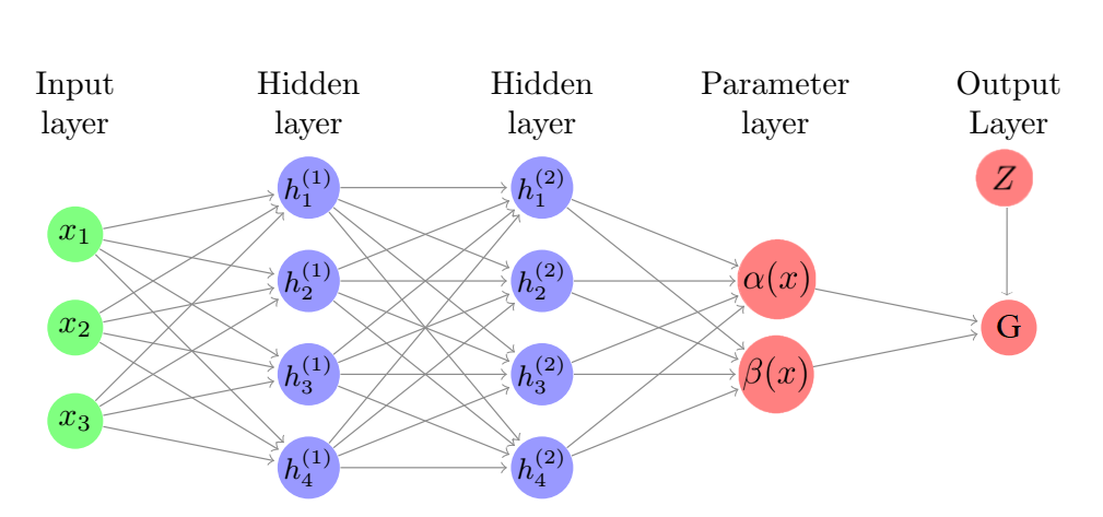
In Farrell, the authors posit that $$\mathbb{E}\left(Y\mid X=x, Z=z\right)=G\left(\alpha(x)+\beta(x)z\right)$$ where $G(u), u\in \mathbb{R}$ is a known link function specified by the researcher, and $\alpha(\cdot)$ and $\beta(\cdot)$ are unknown functions to be estimated. Since we are interested in effects of $Z$ on a real-valued $Y$, we use an identity link function so that $G(\cdot)$ can be removed from the equations and we have $$\mathbb{E}\left(Y\mid X=x, Z=z\right)=\alpha(x)+\beta(x)z.$$ The authors propose estimating $\alpha(\cdot)$ and $\beta(\cdot)$ with one deep fully connected neural network. We implement this architecture as a fully connected neural network with two hidden layers and a two-node parameter layer which outputs $\alpha(X)$ and $\beta(X)$. The output of this architecture is then a linear combination of the two nodes in the parameters layer, $\alpha(x)+\beta(x)z$.

The figure below is a pictoral representation of how the Farrell method works.

The Farrell method with a 3-dimensional vector of covariates $X$, 4
nodes in each hidden layer (in practice, these layers are usually much
deeper). $G$ is an activation function that takes $\alpha(X)+\beta(X)Z$
as an argument. — **Figure 1**: The Farrell method with a 3-dimensional vector of covariates $X$, 4 nodes in each hidden layer (in practice, these layers are usually much deeper). $G$ is an activation function that takes $\alpha(X)+\beta(X)Z$

Since $Y$ is real-valued, we use mean squared error (MSE) as a loss function in training each of the methods introduced in this section.

BCF-nnet

Based on the results and discussion in BCF, we hypothesize that splitting $\alpha(\cdot)$ and $\beta(\cdot)$ into separate networks with no shared weights may yield better CATE estimates on some data generating processes (DGPs). The BCF nnet method specifies $$\mathbb{E}\left(Y\mid X=x, Z=z\right)=\alpha\left(x, \hat{\pi}(x)\right)+\beta(x)z.$$ In BCF, $\alpha$ and $\beta$ are given independent BART priors. $\hat{\pi}(x_i)$ is an estimate of the propensity function. We implement the BCF nnet architecture as in the figure below: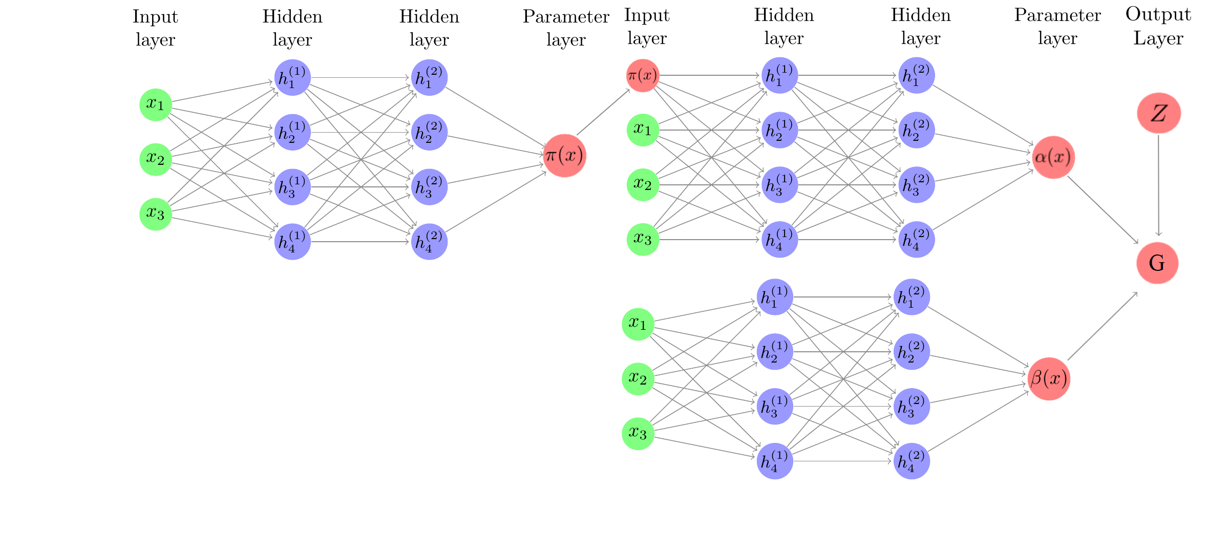

While the shared-weights versus separate weights distinction between Farrell and BCF nnet has been made clear, a subtle difference between the architectures is that BCF nnet allows for an estimate of the propensity function to be incorporated as a feature in the $\alpha(X)$ network. Since targeted selection implies $\alpha(X)$ is a function of $\pi(X)$, this parameterization was observed to be helpful in BCF.

Separate Network Regression Approach

The "naive" method in our comparison employs two completely separate regression models, $$Y_1(X) = \mathbb{E}\left(Y \mid Z=1, X\right) \text{ and } Y_0(X) = \mathbb{E}\left(Y \mid Z=0, X\right) $$ With these two regression functions, our estimate of $\beta(X)$ is simply $\beta(X) = Y_1(X) - Y_0(X)$. Each $Y_i(X)$ is constructed as a 2-layer fully connected neural network, with the number of parameters chosen to be similar to the number chosen for the Farrell and the BCF architecture.

Linear Model

We also compare our two neural network architectures to a simple linear model's estimate of $\beta$ $$Y=\beta Z+X\delta +\varepsilon$$ where /)\beta/) is the coefficient of interest and represents the average treatment effect. The model is fit using ordinary least squares (OLS). We allow for interaction effects between /)X/) and /)Z/).

Simulation Summary

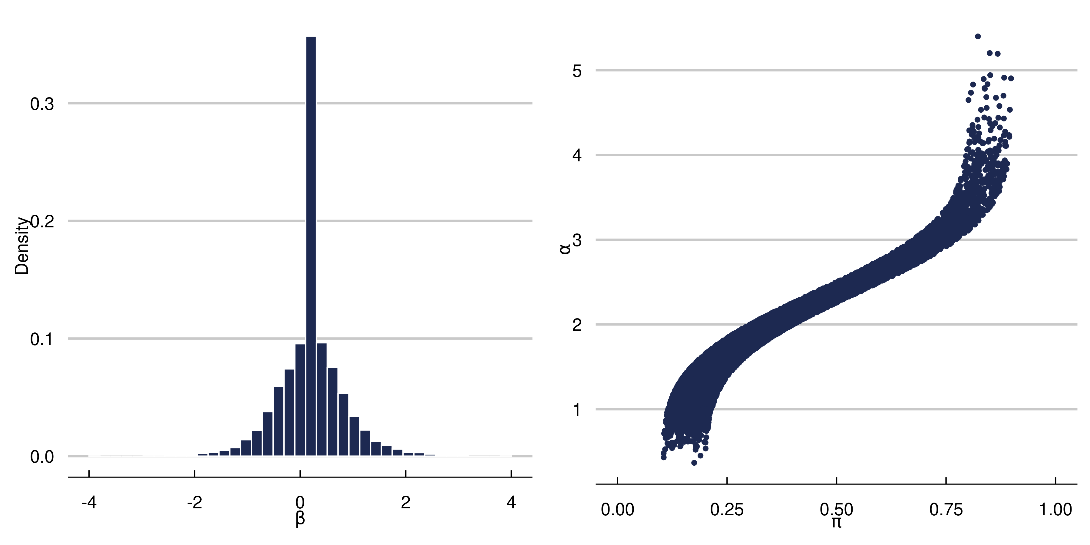
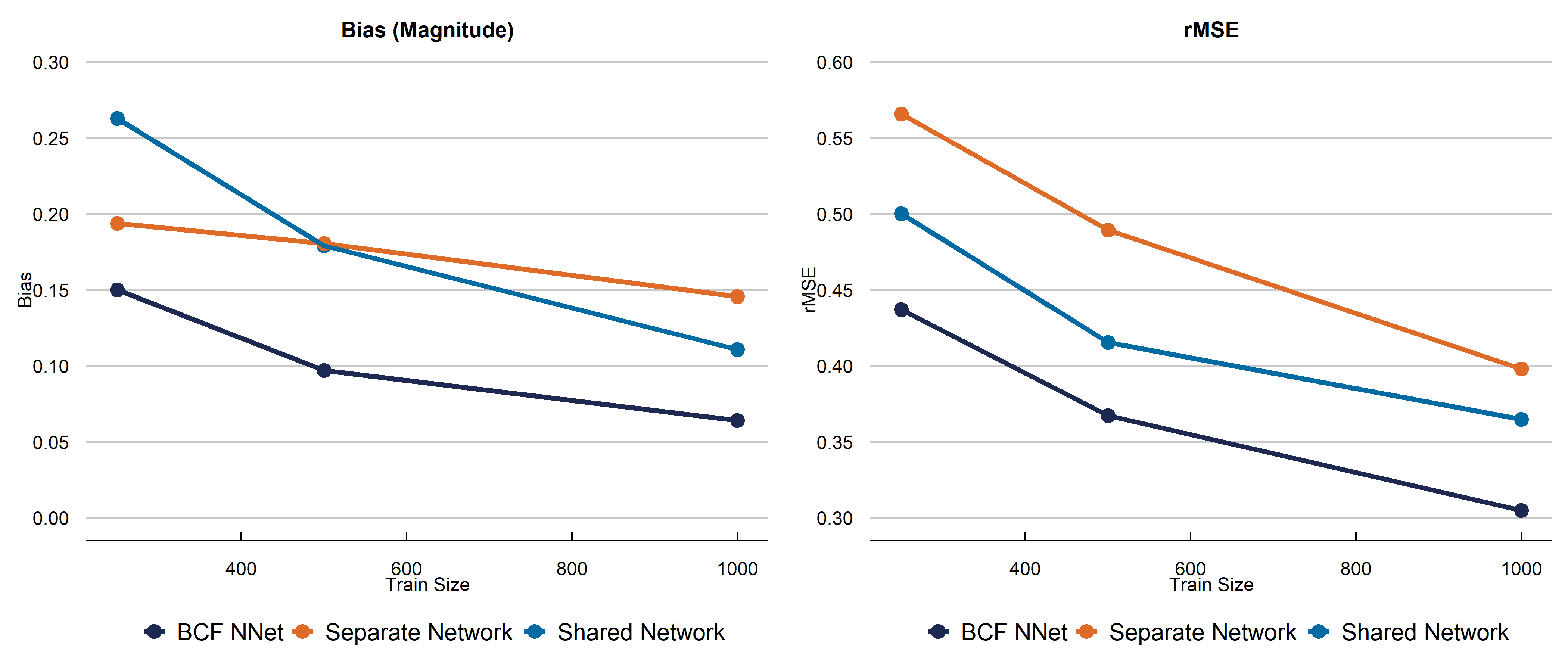
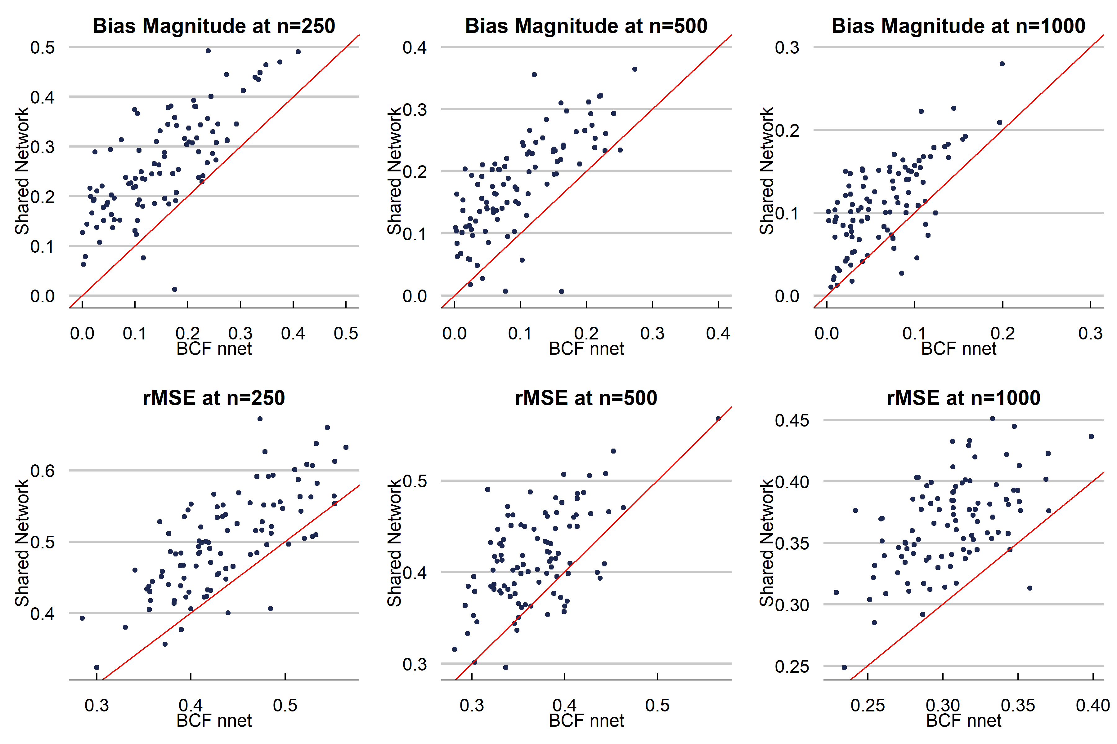
Below is the first DGP we run. We choose a complex function for $\alpha$ and strong targeted selection, and a simpler function for $\beta$ (which allows for heterogeneous effects) to illustrate the effect of targeted selection. $$ \begin{aligned} \begin{split} X_1, X_2, X_3&\sim N(0,1)\\ X_4&\sim \text{binomial}(n=2, p=0.5)\\ X_5 &\sim \text{Bern}(p=0.5)\\ X &= \left(X_1, X_2, X_3, X_4, X_5\right)\\ \beta\left(X\right) &= \begin{cases} 0.20+0.5X_1\cdot X_4& \text{small treatment to prognosis ratio}\\ \end{cases}\\ \alpha\left(X\right)&=0.5\cos\left(2X_1\right)+0.95*|X_3|\cdot X_5-0.2X_2+1.5\\ \pi(X) &= 0.70\Phi\left(\frac{\alpha(X)}{s(\alpha(X))}-3.5\right)+u/10+0.10\\ u&\sim \text{uniform}(0,1)\\ Y&= \alpha(X)+\beta(X)Z+\sigma\varepsilon\\ \varepsilon &\sim N(0,1)\\ \sigma &= \text{sd}(\alpha(X))\cdot \kappa \\ Z &\sim \text{Bern}(p=\pi(X)) \end{split} \end{aligned} $$ We choose the total number of parameters in the Shared architecture to be about the same as the separate network ($\alpha$ + $\beta$ networks). In the Shared network, this means we have 100 hidden nodes in layer 1, and 26 in layer 2, meaning 3,280 total parameters.

In the BCF nnet architecure, we have 60 parameters in the $\alpha$ first layer, 32 hidden nodes in the second layer. For the $\beta$ network, we have 30 and 20 hidden nodes respectively. This yields 3,226 total parameters. For both methods, we use a learning rate of 0.001 with an Adam Optimizer, we use Sigmoid activation, binary cross entropy loss for the propensity, MSE for the other networks, ReLu activation (double check), 250 epochs, and a batch size of 64. The dropout rate is 0.25 in every layer. The propensity score for the BCF NNet architecture is estimated using a 2 layer fully connected neural network with 100 and 25 hidden nodes respectively, and the rest of the parameters the same as above. In the separate network approach, we build the architecture separately using a 2-layer fully constructed neural network (for both $Y_1$ and $Y_0$ infrastructure with 50 hidden nodes in layer 1 and 26 in layer 2 for both models. This is a total of 3,306 parameters. The other hyperparameters are the same as the BCF NNet and Shared Network approach. Below is a figure summarizing the effect of our data generating process. The graphs indicate we should be witnessing strong RIC, making this is a fairly difficult CATE estimation problem.

On the left panel is a histogram of /)\beta/). On the right is a plot of $\alpha(X)$ vs $\pi(X)$, indicative of strong targeted selection. For this particular realization of our DGP, with $n=10,000$, the mean of $\beta(X)=0.20$, the mean of $\alpha(X)=1.95$, and the range of $\pi(X)=\left(0.11, 0.90\right)$, with mean of 0.37. — **Figure 3**: On the left panel is a histogram of $\beta$. On the right is a plot of $\alpha(X)$ vs $\pi(X)$, indicative of strong targeted selection. For this particular realization of our DGP, with $n=10,000$, the mean of $\beta(X)=0.20$, the mean of $\alpha(X)=1.95$, and the range of $\pi(X)=\left(0.11, 0.90\right)$, with mean of 0.37.

The figure below compares a summary of biases and rmse's across the 100 Monte Carlo runs for the shared and BCF-nnet architectures.

**Figure 4**: We run the DGP described above with $\kappa=1.0$ across 100 independent trials (varying $\varepsilon$) for each size $n$. We generate $X$ for each size $n$, but keep the $X$ matrix the same for each of the 100 independent trials for each sample size (i.e. the $X$ vary across the sample sizes, but are constant at each iteration per sample size). We train on the $n$ size, but test on a size of 10,000, to ensure we are looking at population parameters. The **true** value of the treatment effect is about 0.20.

Finally, the figure below gives a more comprehensive image by comparing individual biases and rmse's across the 100 Monte Carlo runs for the shared and BCF-nnet architectures.

**Figure 5**: Comparing Individual biases and rmse's across the 100 Monte Carlo runs for the shared and BCF architectures. Dots above the line indicate worse performance.

Discussion

We presented a new neural network architecture built off the structure of the well-known Bayesian Causal Forest algorithm specifically to estimate causal effects. While a fully connected neural network is not our recommended choice of model for fitting tabular data, we demonstrate improvements on existing neural network causal effect estimators using this structure. Further work includes altering the acrhitecture chosen to model the prognostic and treatment functions. Stay tuned!

Acknowledgements

We thank ASU Research Computing facilities for providing computing resources.

References

Hahn, P.R., Murray, J., & Carvalho, C. (2020). Bayesian Regression Tree Models for Causal Inference: Regularization, Confounding, and Heterogeneous Effects (with Discussion). Bayesian Analysis, 15(3), 965-1056.

Farrell, M., Liang, T., & Misra, S. (2020). Deep Learning for Individual Heterogeneity. arXiv preprint arXiv:2010.14694.

Wager, S., & Athey, S. (2018). Estimation and Inference of Heterogeneous Treatment Effects using Random Forests. Journal of the American Statistical Association, 113(523), 1228-1242.

Krantsevich, N., He, J., & Hahn, P.R. (2021). Stochastic Tree Ensembles for Estimating Heterogeneous Effects. Arxiv Preprint.

Hill, J. (2011). Bayesian Nonparametric Modeling for Causal Inference. Journal of Computational and Graphical Statistics, 20(1), 217-240.

Cybenko, G. (1989). Approximation by superpositions of a sigmoidal function. Mathematics of control, signals and systems, 2(4), 303-314.

Hernan, M., & Robins, J. (2020). Causal Inference: What If. Boca Raton: Chapman & Hall, CRC.

Chipman, H., George, E., McCulloch, R., & others (2010). BART: Bayesian additive regression trees. The Annals of Applied Statistics, 4(1), 266-298.